Images
How do you represent a photograph? You could say pixels, but originally, there were no pixels in photographs. Therefore, we could say an image is a function that maps spatial location to intensity, where intensity is a number between 0 and 1, inclusive:
$$f : \mathbb{R}^2 \to [0, 1].$$
What about color images? We could extend the function definition to one using RGB:
$$f : \mathbb{R}^2 \to [0,1]^3.$$
This definition is great by itself, but computers cannot represent arbitrary functions. Therefore, digital images record only intensities/colors at a finite grid of locations. Thus, grayscale images are 2D arrays while color images are 3D arrays. On the same note, pixel values are not real numbers but rather integers between 0 and 255 (but this is not always the case).
Image Processing
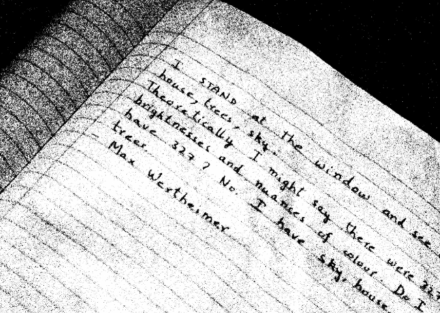
One task we might want to complete is to convert a picture of a notebook into a text document. This requires us to recognize each letter, but how do we know where the letters are?
Recall that images are functions. thus, grayscale images are functions $f : [a,b] \times [c,d] \to \mathbb{R}$. Therefore, we can use a threshold:
$$f’(x,y) = \begin{cases} 1 & f(x,y) > 122 \\ 0 & f(x,y) \leq 122. \end{cases}$$
Blurring
Suppose we take a photo in the dark. How do we fix this? By adding a constant to the function, the image gets brighter, but there still isn’t much contrast.
To increase contrast, we could multiply $f$ by a constant, but this increases noise:
First, we can assume that noise is independent of other locations and distributed according to a Gaussian distribution. Technically, low-light photography is not, but that is another story.
We can also use a nice fact about the real world: close areas in real life have similar intensity values. Therefore, we can replace each pixel’s value with the average of its neighbors. You can choose neighborhoods of different sizes, e.g. $3\times3$ or $5\times5$. However, neighborhoods that are too big can cross boundaries, and you can lose information despite getting rid of more noise. This technique is called mean filtering. A $3\times3$ mean filter would look like
$$S[f](m,n) = \sum_{i=-1}^1 \sum_{j=-1}^1 f(m+i,n+j)/9.$$
Mean filtering only slightly changes the appearance of noisy images, but it can be impactful when thresholding.
We can add a weight and generalize the neighborhood size:
$$S[f](m,n) = \sum_{i=-k}^k \sum_{j=-k}^k w(i,j) f(m+i,n+j).$$
Here, the weight $w$ accounts for the actually division in the mean. For a mean filter, $w(i,j) = 1/(2k+1)^2$.
If $w(i,j) \geq 0$ and sum to 1, then we have a weighted mean filter. On the other hand, if we let $w(i,j$) be arbitrary real numbers, then there becomes a correlation between certain areas of different neighborhoods, which we call cross-correlation.
What happens at the image boundary? At the top left pixel, can cannot take an average including a pixel above and to the left of that pixel since such a pixel doesn’t exist.
One approach we could take is to not compute an average for boundary pixels, shrinking the new image. This is called valid cross-correlation, and the output image has size $m-k+1$.
Alternatively, we could treat non-existent pixels as having a certain value, like 0, and maintain the original size. This is called same cross-correlation. However, we could also compute averages for pixels outside of the original image, making the new image larger. This is called full cross-correlation and results in an output image of size $m+k-1$.
Convolution and Cross-Correlation
Cross-correlation is defined as
$$w \otimes f (m,n) = S[f](m,n) = \sum_{i=-k}^k \sum_{j=-k}^k w(i,j) f(m+i,n+j),$$
while convolution is defined as
$$w * f(m, n) = S[f](m,n) = \sum_{i=-k}^k \sum_{j=-k}^k w(i,j) f(m-i,n-j),$$
Importantly, cross-correlation (and convolution) is linear in both $w$ and $f$.
Additionally, cross-correlation follows shift equivariance, so shifting then filtering is the same as filtering then shifting.
Cross-correlation and convolution are similar operations and have similar properties, but they are just weighted differently.
Sharpening
When we blur images, we are changing the values of each pixel. If we undid those changes on the original picture, we could get a sharper image:
$$f_{sharp} = f + \alpha(f-f_{blur}).$$
Can we make a filter to do this? Simplifying the above gives
$$\begin{aligned} f_{sharp} &= f + \alpha(f-f_{blur}) \\ &= (1+\alpha)f-\alpha f_{blur} \\ &= (1+\alpha)(w*f) - \alpha(v * f) \\ &= ((1+\alpha)w - \alpha v) * f, \end{aligned}$$
where $w$ is the identity filter and $v$ is a blurring filter. The last line follows from linearity.