Convolution
Last class, we mentioned that we can use convolution to turn color images gray. To do this, we can treat a color image as three layers of grayscale images and use a three-layer kernel.
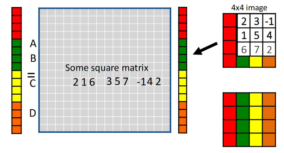
We also mentioned looking at 1D convolution as matrix multiplication. To extend this to 2 dimensions, we can simply put all the rows/columns of the image in one long column vector, doing the matrix multiplication, and unwrapping the long column vector back into an image. Although it requires thinking to squish the kernel and place it into the square matrix, it works out.
Geometric Transformations
Geoemtric transformations have the form
$$\begin{bmatrix} x^\prime \\ y^\prime \end{bmatrix} = T\left(\begin{bmatrix} x \\ y \end{bmatrix}\right).$$
One example of a geometric transformation is zooming in, which is a common action people take. Another is rotation followed by translation.
One important concept is differentiating forward transformations and inverse transformations. Sometimes, transformations don’t map to certain positions, so doing the inverse results in blank spots.
If $(x,y)$ goes to $(x^\prime, y^\prime)$, then we can say $f^\prime(x^\prime, y^\prime) = f(x,y)$. But must $x,y,x^\prime,y^\prime$ be integers? They don’t have to be, but we must somehow interpret non-integer results in a way to put them in an image with integer pixels.
One solution is nearest neighbor interpolation, in which pixels take on the value of the nearest output value. This method does not produce that great results.
Another solution is bilinear interpolation, in which we weight the four nearest pixels such that their weighted average is the output pixel:
$$\begin{aligned} g(x,y) =& Cf(x_l,y_l) \\ &+ Bf(x_h,y_l) \\ &+ Af(x_h,y_h) \\ &+ Df(x_l,y_h), \end{aligned}$$
where $A,B,C,D$ are (normalized) rectangle areas.
Gaussian interpolation is another method.
Interpolation can also be used for upscaling images. When using nearest neighbor interpolation, we will often see blocky effects. Bilinear interpolation works a lot better although it may seem blurry.
What if we want to zoom out (downsample), e.g. by a factor of 2? One way to do this is to drop every other pixel, in which case interpolation is not needed. However, this can cause weird patterns to emerge, which we call aliasing. This happens because in the original image, there can be many thinly separated regions of different colors, and when pixels in between are removed, those separations could disappear. This also appears in signal processing when interpolation of a high frequency wave could cause us to infer a low frequency wave.
The solution to aliasing in signal processing is the Fourier transform, in which functions are decomposed into sines and cosines. We can do something similar by blurring (using Gaussian pre-filtering) the original image to preserve the relations between dark and light pixels.
One neat thing we can do with this is blurring then subsampling repeatedly to get different information about the image.