Bilinear Interpolation Review
To perform bilinear interpolation, we could use the traditional area formula, or we could use one linear interpolation to find points on the edge that lie across from each other through the point of interest and perform another interpolation to get the value of the point we want.
Grouping and Edges
Why grouping? As humans, when we see images or moving pictures, we don’t look at pixels, we see objects that the pixels represent. Therefore, it is useful to have computers do the same thing.
How do we look for edges? We could say edges are curves in the image across which brightness changes a lot. However, lighting conditions may make it so that the brightness does not change a lot across it. There are several types of edges:
- Depth discontinuities
- Normal discontinuities
- Discontinuities in “paint”
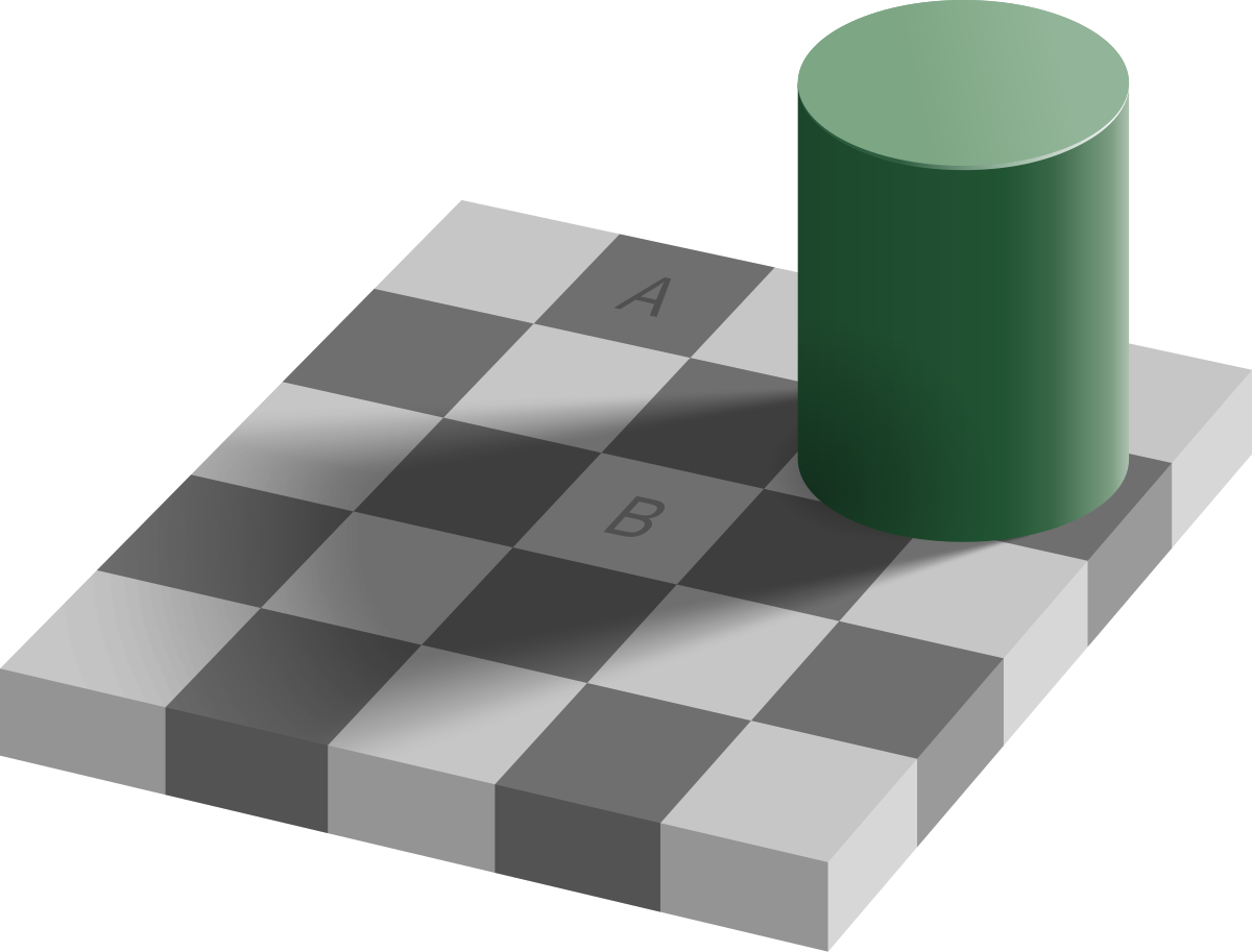
- Shadows
To find images, we can look at the intensity function along a line and find where it changes quickly, which is where the magnitude of the derivative is high. Importantly, differentiation is linear and shift-equivariant.
But how can we take a derivative of an image, which is discrete rather than continuous? We have two options:
- Reconstruct a continuous function for the image.
- Compute a slope rather than a limit of a slope as the derivative.
How would we implement the latter as a linear filter? We can do it like so in the $x$ direction:
$$ \begin{array}{|c|c|c|} \hline 0 & 0 & 0 \\ \hline 1 & -1 & 0 \\ \hline 0 & 0 & 0 \\ \hline \end{array} $$
We can do something similar for the $y$ direction.
How does noise affect edge detection? If the intensity function is noisy, then its derivative will be very spiky, and it won’t be clear where the edge is. The solution is to use a Gaussian to smooth out the image, and the edge will become more apparent.
Since convolution is associative, we can use the fact that
$$\frac{d}{dx} (f * h) = f * \frac{d}{dx} h,$$
which can save on computation. However, as discussed in a previous lecture, the $\sigma$ of the Gaussian changes what scale edges are detected, so we will later study how $\sigma$ affects this.
So far, we have been doing the Gaussian in two dimensions. But should we be smoothing along the edge to the same degree that we smooth across it? In practice, probably not, which is why we use an anisotropic Gaussian which has a lower standard deviation along one direction.